Full (CaRT) Decision Tree Example
This post was written as supplementary material for the Machine Learning course.
This example (borrowed from here) will walk through the steps of building a decision tree using the CaRT algorithm. I made my own small little adaption, let’s go through that one first, then after hopefully the video adds a bit more information.
Our Data
Say we have the following dataset with Belgian beers, they have a color (Black, Red, and Yellow), alchohol by volume (ABV) category, and a label (type of beer). Remember that when running a decision tree, at each step we try to a) find the most effective question by which to split our data, b) partition our data in branches according to this question, and c) keep repeating this until the impurity of the final split is 0 (or we meet some other stopping condition, such as tree depth).
| color | ABV | label |
|---|---|---|
| B | 3 | Stout |
| Y | 3 | Stout |
| R | 1 | Ale |
| R | 1 | Ale |
| Y | 3 | Trip |
X, y = [[data]], [labels]
impurity = 1
for yi in set(y):
    # calculate prob of label yi in y
    # calculate impurity of yi
    impurity -= prob ^ 2
Calculate Impurity
For step a) we need two things: we need to calculate the probability for a label $y_i \in Y$ given any (sub) set of our data $X$, and the impurity of our split (using those probabilites), using the following formula for Gini (note that the formulation for Gini in the code snippet above is the same as the lecture slides). I will refer to $X$ as $D$ to avoid ambiguity; $D_p$ will be the data split of a parent node (at the top this is all of $D$), and $D_j$ that of the $j$th child node (so given binary classes we can have either $D_\text{left}$ or $D_\text{right}$. Our Gini $G_I$ for a particular class $c$ at node $t$ is then:
\[I_G(t) = \sum^c_{i=1} p(i|t) \cdot \big(1 - p(i|t)\big) = 1 - \sum^c_{i=1} p(i|t) \cdot p(i|t) = 1 - \sum^c_{i=1} p(i|t)^2\]Look at the code above, and relate the last part of the formula to the code there. Let’s try this for our root node (our original dataset) first:
\[I_G(D_\text{root}) = 1 - 2/5^2 + 2/5^2 + 1/5^2 = 0.64\]Split Our Data
Now let’s start by asking one question, namely: color == black?. We get two branches with the following data:
| color | ABV | label |
|---|---|---|
| Y | 3 | Stout |
| R | 1 | Ale |
| R | 1 | Ale |
| Y | 3 | Trip |
| color | ABV | label |
|---|---|---|
| B | 3 | Stout |
Now if we again calculate $I_G(D_{\text{left}})$ and $I_G(D_{\text{right}})$ we get:
\[1 - 1/4^2 + 2/4^2 + 1/4^2 = 0.625\]… and:
\[1 - (1/1)^2 = 0.0\]Calculate Information Gain
To calculate what the Information Gain of this particular question is, we generally we use the average impurity (or average Gini Index) formulation of Information Gain ($IG$):
\[IG(D_p, f) = I_G(D_p) - \frac{N_\text{left}}{N} \cdot I_G (D_\text{left}) - \frac{N_\text{right}}{N} \cdot I_G (D_\text{right})\]Note that $IG$ (Information Gain) and $I_G$ (Gini) are different!
Where $f$ is the feature (or you can say $q$ for question) on which we split our data. Basically, we just fill in what we have until now, where in the first part $I_G(D_p) = I_G(D_\text{root})$, so:
\[IG(D_p, \texttt{Color == Black}) = 0.64 - 4/5 \cdot 0.625 - 1/5 \cdot 0 = 0.144\]Determine Best Split
If we repeat this a bunch more, we get the following Information Gain for all possible questions:
| Question | $IG$ |
|---|---|
color == black | 0.14 |
ABV >= 3 | 0.37 |
color == yellow | 0.17 |
color == red | 0.37 |
ABV >= 1 | 0.00 |
And take:
\[\hat{q} = \arg \max_{q \in Q} IG(D_p, q),\]where $Q$ (or $F$) would be all possible questions. I.e. we take the best question $\hat{q}$ that is the $q$ that maximizes the Information Gain. Given that both ABV >= 3 and color == red give us an equal Information Gain, we will just opt for the first in the list, and start splitting the root note in the tree by this first rule.
Putting It Into Code
Consider the following pseudo-code:
def build_tree(D):
    info_gain, best_feature = find_best_split(D)
    if info_gain == 0: return Leaf(features)
    true_D, false_D = partition(D, best_feature)
    true_branch = build_tree(true_D)
    false_branch = build_tree(false_D)
    return Node(best_feature, true_branch, false_branch)
Note that find_best_split (or best question) is a combination of all sections above. If we end up with a final Information Gain for the current split of 0, it means that there were no more questions to ask, so we stop, and create a Leaf. If not, we use our best question to partition the final tree (split data section), we make sure we recursively call the same function again on the left side of the branch, and the right side (thus making a reference to these in the code), and then we return a Node object.
Visualizing and Continuing our Tree
Now because this is a small tree, we already end up with a pure split with this single question, we just need to ask one more, and we’re done. The full tree and splits are visualized below.
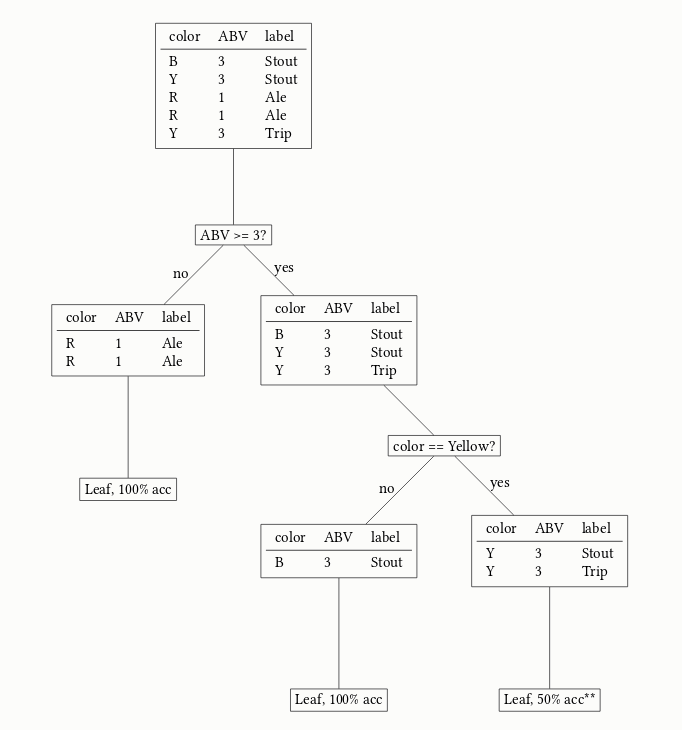
**Given there are no more further questions to ask here, we have to randomly guess between the two labels that we know, giving this leaf’s accuracy only 50%.
Hope that was useful!